
The 2026 edition of MLT-2 is now available for download.
This version includes support for a new custom Navy ERP T-code (ZRMWM0003) which provides all data fields available in the material label.
The 2026 edition of MLT-2 is now available for download.
This version includes support for a new custom Navy ERP T-code (ZRMWM0003) which provides all data fields available in the material label.
After a few years of MLT-2 enjoying a well-deserved retirement, I received a query regarding a user’s inability to use the MLT-2 MS Access version in 64-bit systems. My first impression was to be flattered that someone was still using it. Then I started looking into the problem.
I had not looked at the MS Access VBA code in years, so I first responded that everything should work, since I am able to run the program just fine in my 64-bit Windows 10 machine. It wasn’t until later that I realized my error. Despite Microsoft stating the MS Office installs in 64-bit by default, I was running the 32-bit version of Office in my MS Access development machine. So, after correcting that, I was able to replicate the 64-bit error.
After a few hours of tweaking the code to VBA 7 and testing, I had a new version of MLT-2. Along the way, I decided to also ditch the whole subscription model, but keep the expiration date on the releases for ease of support. This way, outdated versions don’t linger in the wild.
There are no new features, but the experience of getting back to doing some development, got me motivated to consider some enhancements. So, let me know what you think. The download links for the refreshed 32-bit and 64-bit versions are below.
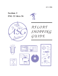
I have had these in my archives for a while, and the publications might be a bit dated, but I thought I would post them here in case anyone finds them useful.

I have been asked about statistical inventory sampling so many times that I felt that I should share my thoughts in an article (or many). In simple terms, statistical sampling is the selection of a subset of items to represent a population and it is a very useful tool for establishing inventory accuracy.
In order for the process to be considered representative, there are a few fundamental rules:
The following are some common terms you would encounter: confidence level, sample size, population size, margin of error. The vast majority of the time, the confidence level and margin of error will be dictated to us, as this determines the precision and robustness of our results. A very common set of parameters typical in DoD supply chain policy is 95% confidence level with a +/- 2.5% margin of error.
If talking about confidence levels and margins of error is still fuzzy, fear not, there are tools that make the whole thing practically plug-and-play. I even developed my own spreadsheet calculator in one of my articles on my website (link here).
Note: if you, like me, are “of a certain age” in Navy Logistics terms, you might remember a program called STATMAN that for many years was the Navy’s standard tool for these calculations when dealing with inventory accuracy.
In order to conduct what is called “Simple Random Sampling” there are only a few computations that we need to make: 1) the sample size, and 2) the accuracy results (usually a percentage or ratio). We were going to compute the accuracy anyway regardless of method, so that leaves the sample size as the only new thing we need to figure out. To get the sample size, simply plug the following parameters into the spreadsheet calculator linked in the previous paragraph (or an online tool like this one): 1) population size, 2) confidence level, and 3) margin of error. This will give you the minimum sample size that needs to be collected in order to satisfy the parameters. Select that number of items at random from the population – you can do this manually or using most spreadsheet programs. Then conduct the inventory and compute the accuracy percentage. Whatever percentage you get (e.g. 93%) would be expressed in terms of a “confidence interval”, which is nothing more than stating the margin of error with our results (e.g. 93% +/- 2.5%). That’s it!
Now, like anything, it can get much more complicated. There are sampling strategies that involve stratification, different allocation methods, etc. that are well beyond the scope of this article. Therefore, we will leave things here for now and I hope that you found this article useful.
If you would like to dive a little deeper into the statistics involved in this type of sampling, there is an excellent video in the zedstatistics channel in YouTube titled “What are confidence intervals? Actually” that I highly recommend.
References and further reading:
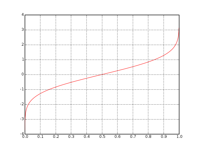
This is a follow-up to my previous post where I detailed my adventures trying to implement in Visual Basic .NET the Inverse Normal Cumulative Distribution Formula (a.k.a. NORMSINV).
As I mentioned in that post, I had been looking for a way to implement the NORMSINV function into a .NET application. I explained how I adapted Peter Acklam’s algorithm for which I adapted some C++ code that I found on the Internet into my .NET application. Later I found that others had done adaptations for various other languages including C#.
Sadly, though Acklam’s algorithm worked well, I could not get the function to match precision closely enough to my legacy program that I was replacing.
Peter Aklam never published his algorithm in any peer-reviewed journals so, other than some historical web pages, it was not possible to follow up to see if any changes or progress took place. However, those historical pages pointed me to the previous work of others.
Conducting that literature research, I found the seminal paper “Algorithm AS 241: The Percentage Points of the Normal Distribution” by Michael J. Wichura (1988), Applied Statistics, vol. 37, pp. 477-484. This paper included an implementation of a function “to compute the percentage point zp of the standard normal distribution corresponding to a prescribed value p for the lower tail area” in FORTRAN. Wichura’s algorithm itself extends previous work by Beasley, J. D. and Springer, S. G. (1977), “The percentage points of the normal distribution”, Applied Statistics, vol. 26, pp. 118-121, which introduced the function PPND (Percentage Points of the Normal Distribution) as part of algorithm AS 111, also published in FORTRAN.
After a quick crash-course in FORTRAN syntax, I was able to easily (but tediously) translate Wichura’s algorithm to Visual Basic .NET. Wichura published two versions of the algorithm in his paper. I only adapted the double-precision function called PPND16 that you can freely download from my github repository.
Since Wichura’s code is published work and all I did was essentially translate it, I am not making any claims to this code other than as a humble contributor. Please feel free to copy or modify it and I hope you find it beneficial.
(Note: Support for MLT-2 will end on 30 September 2022)
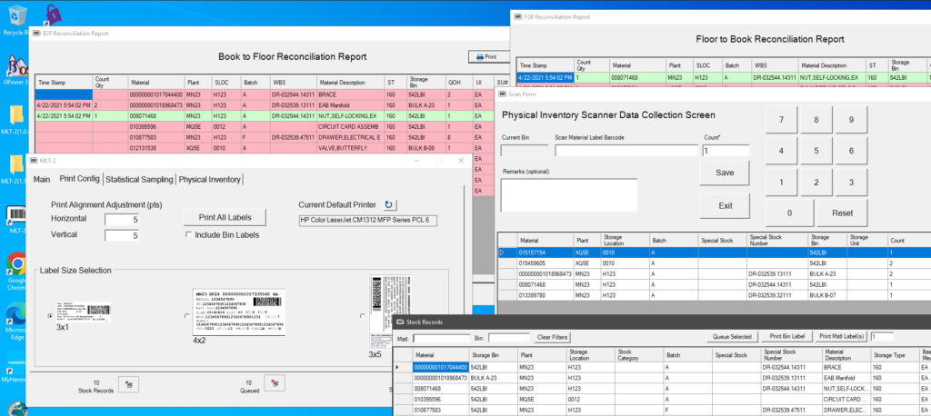
This past Summer we conducted a series of statistical sampling inventories, which caused me to take a look at the Material Label Tool as a starting point for that project. I added some statistical sampling functionality and actually started calling it STATMAN II because it incorporated many of the features of the original STATMAN.
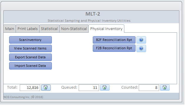
So I have decided to fully evolve the tool into a complete physical inventory data collection utility with full scanning and parsing capability of Navy ERP material labels.
Now that the application is done, I decided to drop the STATMAN II name and am simply calling it MLT-2, or Material Label Tool 2nd generation since it does much more than labeling now.
Who knows? It might come in handy one day.
Update: I have added a page on the main site with a demo video and more information. See it here.

Readers might remember my previous article on counting methods and RFID where I promised to revisit this topic. Well, here we are.
Interest in using RFID for warehouse physical inventory management continues to be high. The technology is very attractive and it is not difficult to wonder why it has taken so long to adopt RFID at this level. Let’s explore the challenges:
This article is only a superficial discussion of the many issues facing RFID adoption for DoD warehouse physical inventory management. There are likely more areas that can be included. As usual, the issues are not all technological. Much more analysis needs to be conducted on the potential for business re-conceptualization in DoD enabled by RFID technology; until then, RFID will remain a technological solution looking for a business problem.
References
Bouet, M., & Dos Santos, A. L. (2008, November). RFID tags: Positioning principles and localization techniques. In Wireless Days, 2008. WD’08. 1st IFIP (pp. 1-5). IEEE.
Gaukler, G. M. (2011). Item-level RFID in a retail supply chain with stock-out-based substitution. IEEE Transactions on Industrial Informatics, 7(2), 362-370.
Hackenbroich, G., Bornhövd, C., Haller, S., & Schaper, J. (2006). Optimizing business processes by automatic data acquisition: RFID technology and beyond. In Ubiquitous and pervasive commerce (pp. 33-51). Springer, London.
Hellström, D., & Wiberg, M. (2010). Improving inventory accuracy using RFID technology: a case study. Assembly Automation, 30(4), 345-351.
I first considered writing an article to discuss strictly MIL-STD 1916, Department of Defense Test Method Standard: DOD Preferred Methods for Acceptance of Product (see PDF file attached to this article). That standard replaced MIL-STD 105 and it is often quoted when discussing statistical sampling, but often with unrealistic expectations. I know what you are thinking, another statistical sampling article? I just can’t seem to get away from the subject. Anyway, I started to dive into the standard in order to explain how it is most useful and when it is more appropriate to stick to general, and more basic, statistical methods when I found myself reading about reliability engineering.
Do reliability engineering concepts apply to inventory accuracy? Do they apply to any business process? It turns out that they can, and there are concepts such as Markov Decision Process (MDP) that are often applied to business.
If we consider physical inventory control as our system, then we can see how that system exists in one state at a time that depends on a previous state (like a Markov chain). The system, most of the time, relies on transactions that themselves have a probabilistic outcome that would have an effect on the state of our inventory. For instance, if 2% of receipts and issues posted are in error.
This brings back some memories. I once wrote a paper on how a logistics information system can impact operational readiness (Ao) and how optimizing the information system could have a more beneficial impact on operational readiness than increasing the reliability of individual weapons systems, because improving Mean Logistics Delay Time (MLDT) improves Ao for all associated weapons systems, even those that have not yet been invented.
It is the same concept with physical inventory controls. The system for managing the inventory, including transactions, policies, and procedures can have a more significant impact on inventory accuracy than any other physical attribute or strictly inventory-related activity.
What does that mean exactly? That there are other blocks in the chain that we need to consider. For example, procurement transactions, database maintenance actions, etc.
So what does that mean for MIL-STD 1916? Although it would not be wrong to apply MIL-STD 1916 to statistical physical inventory sampling to measure accuracy, one would still have to get their hands dirty (sort to speak) in order to analyze and extrapolate the results in a way that they provide us with a measure of our inventory accuracy for our entire population. In order to measure our results to see if we meet DoD guidance, we would still need to compute sample size, margin of error, and confidence intervals using basic statistical processes, even if relying on tables and methods from MIL-STD 1916. That military standard lends itself more to what engineers and reliability analysts refer to as “zero accept, one reject” methods (see this paper by Al-Refaie and Tsao (2011)).
So, to tie back to the MDP concept, MIL-STD 1916 absolutely has a place in physical inventory controls, but most especially in evaluating the reliability and acceptability of the transactional processes that are part of our inventory reliability chain. In other words, testing each block in the chain of processes that affect inventory, such as receipt, issues, transfers, etc. is an excellent application for this type of statistical analysis.
Book recommendation of the month. Well, not really a recommendation, but a suitable reference to the above article: Modeling for Reliability Analysis: Markov Modeling for Reliability, Maintainability and Supportability by Jan Pukite & Paul Pukite. Buy a used copy for $10, the book is not worth the full sticker price.
Recently, I have noticed an increased interest in questioning the validity of conducting statistical sampling inventories. Many people do not understand the concepts or the value of statistical sampling and that may be driving these perceptions.
This post includes some excerpts from a paper that I wrote some years ago. It establishes the relationship from the CFO Act of 1990 down to DoD guidance on the conduct of statistical sampling inventories.
The Chief Financial Officer’s (CFO) Act of 1990 (Public Law 101-576) Established Statutory Reporting Requirements Regarding Inventory and Assets under the Authority of the Agency’s CFO
The CFO Act of 1990 provides the statutory requirements that:
The Federal Financial Management Improvement Act (FFMIA) of 1996 (Public Law 104-208) Established Specific Statutory Audit Requirements
DoD Financial Management Regulations (FMR) implement Public Law 104-208 (FFMIA of 1996) and 101-576 (CFO Act of 1990)
The DoD 4140.1-R Establishes Policies for Physical Counting and Gives Priority to Sampling Methodologies
The DoD 4000.25-M Vol 2 Establishes Procedures for the Conduct of Statistical Sampling Inventories
References
I have come to the conclusion that there are simply no good books on statistical sampling for novice practitioners. A lot of the literature begins by covering statistical principles, which is important, but statistics is such a large field that most people get turned off or lost. There is also a lot about the field of statistics that we don’t need to know, for our purposes. Which brings me to my latest book recommendation.

“Audit Sampling: An Introduction”, by Dan Guy, Douglas Carmichael, and Ray Whittington, is perhaps the best book that I have been able to find. I have the Third Edition of this textbook and it is the most concise textbook that I have found on the subject. It is laid out precisely for auditors, meaning that there are not too many side-bars into statistical or mathematical theory. It is the closest thing that I have found to a step-by-step guide for audit sampling, although that is not what this book is. It is a textbook, in the traditional sense. It also includes some excellent appendices, such as the full text of Statement of Auditing Standards (SAS) No. 39: Audit Unit (AU) 350 – Audit Sampling.
I recently revisited this textbook while preparing for some discussions for an upcoming project. This inspired me to put together a presentation to try to condense the topic of statistical sampling of physical inventory down to its simplest tasks: Planning, Selection, and Evaluation.
In the Planning phase, we are concerned with establishing the statistical parameters, such as the confidence level and margin of error – which, in many cases, are given to us. We use those parameters during this phase to calculate the sample size (see my previous post).
The Selection phase is concerned with randomly choosing the samples to be tested.
Finally, the Evaluation phase consists of testing the samples, computing the results, and reporting our findings.
I put together a slightly expanded version of the above in my own Sampling Guide, available for download from this link.